
Predicting Property Sale Values in Ames, Iowa
Using regression, random forests, time
Rishi Goutam, Srikar Pamidi, James Goudreault, Akram Sadek
March 10, 2022—15 min readThe Ames housing dataset is famous as an open Kaggle competition and for its use in undergraduate statistics courses as an end-of-term regression projectSee here. Unlike the similar Boston housing dataset, it has a relatively large number of variables81 versus 14 and observations2,580 versus 506. In tackling this problem, we would have to go beyond a simple, automatic algorithm such as stepwise selection, to construct a final model.
In this project, we took on the persona of being a data science team at a made-up local realty firm, Regression Realty, in early 2011. Our stakeholders were primarily our firm’s listing and selling agents and our goals were to:
- Provide insight into Ames’ housing market conditions given that we were just out of a major financial crisis.
- Surface advice they could give to their clients. For instance, tell a buyer a house is overpriced or a seller that they could make some money by remodeling a fireplace.
- Create predictive models that can be meaningfully used in our firm’s mobile or web app. This means not using too many features (agents have to input data) or taking a long time to run a model.
You can find our code and presentation slides on GitHub.
Table of Contents
The Ames dataset
Cleaning
The data comprises information collected from the Ames City Assessor’s OfficeRather than from traditional MLS data sources during 2006—2010 with variables being nominal, ordinal, continuous, and discrete in nature. As a real-world dataset, it required extensive cleaning and feature engineering to be able to garner insights and create models.
We dropped one duplicate observation and removed two outliersWhere GrLivArea > 4,000 feet2 as per the recommendation of the dataset authorDean De Cock. Journal of Statistics Education Volume 19, Number 3. Another approach would have been to define outliers as properties whose sale prices were more than, say, four standard deviations from the mean. This would have dropped five points in our case.
Imputation
We imputed missing valuesFor implementation details, see clean.ipynb for features by taking the mean, median, or mode as applicable of the feature category.
Sometimes, imputation was done by making reasonable assumptions. For instance, a missing GarageYrBlt can be imputed by the year the property was built. Finally, we imputed None (e.g., MasVnrType) or 0 (e.g., MasVnrArea) for values that might not exist or for which an educated guess could not be made.
Feature Engineering
In addition to the given dataset’s features, we added two more we thought might influence a property’s SalePrice:
- The public school district for a property
- Interest rate for the month the property was sold as determined by the 10-year treasury yields from the ^TNX index.
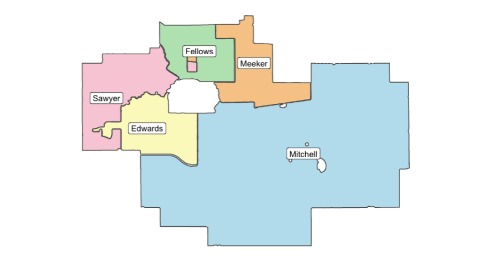
Ames has five school districts and we might expect property value to vary based on the quality of the school. By determining whether a property’s latitude and longitude coordinates fall within the district’s boundaries, we can determine the school district. First, we used geopySee geo_locations.ipynb to query OpenStreetMap’s Nominatim geocoding software to acquire the property coordinates. There are several python and R tools to help solve the point-in-polygon problemSee districts.R. We used R’s sf package.
We also derived features we believed might be useful, such as whether a property is near a park, an arterial road, or a rail line; if it is a Planned Unit Development (PUD), has been renovated, has a pool, the number of floors, etc.
Feature engineeringSee engineer.ipynb was conducted to also
- Ordinalize some categorical features
- (
*Qual,*Cond,Neighborhood, etc)
- (
- Combine multiple features into a single feature
- (
StreetAlley, Total Outdoor foot2, etc)
- (
- Collapse features into smaller set of categories
- (
MSSubClass, etc)
- (
Notable Findings
Comprehensive exploratory data analysis produced a lot of insights and informed feature selection and engineering—here follows the distilled version.
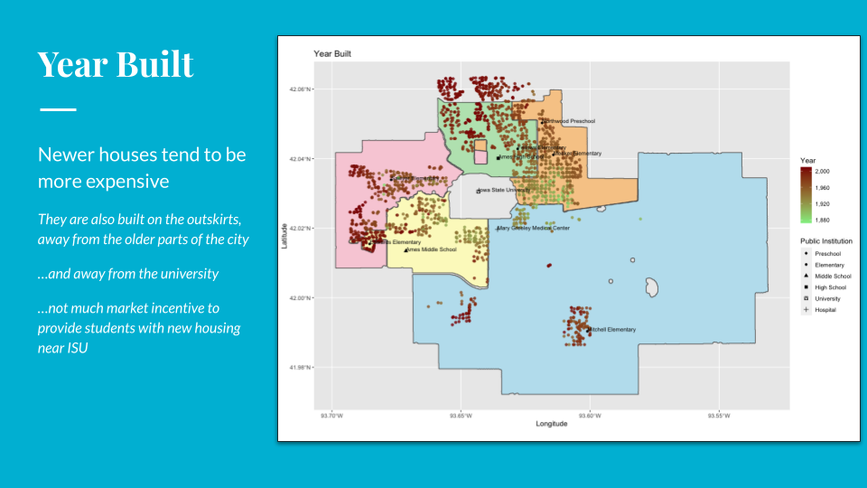
First, we see Ames properties plotted against school districts. We also plot the schools, a hospital, and Iowa State University.

We will later see whether school districts matter (and how much) for a city like Ames. Compared to features such as Neighborhood, we will see that district is not as important.
Still, all that mapping was useful as an EDA tool and to check our assumptions.
Area features display increasing variance as we see below. We see the plots of SalePrice (y) versus GrLivArea (x) as well as the residuals.
We went with a log-linear transformation in our models as it showed a lot of improvement in reducing the “<”-shaped spread in property sale prices. Log-log shows marginal improvement, but is also harder to explain to a layman. When taking a transformation, we must remember to reverse the transformation after our model makes a prediction.

Size matters…in most cases. The price of a single family home is strongly correlated with the number of rooms in the home. Not so with other home types.

Neighborhood is very strongly predictive of price. As they say, location, location, location!
What this means is that we can treat Neighborhood as an ordinal feature in our models.

Market Analysis
In addition to exploring the dataset itself, we wanted to focus on the Ames housing market dynamics. We came in to this with a lot of assumptions—the 2008 crash must have caused house prices to fall. Seasonality patterns in the housing market must change too. Surely, single-family homes would be more resilient than multi-dwelling units to the depressed market conditions?
We used a SARIMA model to look at average SalePrice for the dataset. We split up the properties by quintile to see if there was a difference between expensive and cheap houses.

We can see that in 2006-2010, the house prices by quintile stayed relatively constant. This is counterintuitive, since the housing market collapsed in 2008, and we do not see that reflected in any of the quintiles. Given that we lived through this recession and knew house prices to be falling where we grew up, we were perplexed at what was going on in Ames. We conducted a Ljung-Box testSee code to see if we could reject H0—whether the data are independently distributed. I.e., the correlations in the population from which the sample is taken are zero, so that any observed correlations in the data result from the randomness of the sampling process.
# Ljung-Box Test—We test to reject H_0, looking for p<.05
test1 <- Box.test(pur.ts,type="Ljung-Box", lag= log(nrow(pur.ts))) # p = .99
test2 <- Box.test(o.ts,type="Ljung-Box", lag= log(nrow(o.ts)))     # p = .14
test3 <- Box.test(t.ts,type="Ljung-Box", lag= log(nrow(t.ts)))     # p = .34
test4 <- Box.test(th.ts,type="Ljung-Box", lag= log(nrow(th.ts)))   # p = .94
test5 <- Box.test(fo.ts,type="Ljung-Box", lag= log(nrow(fo.ts)))   # p = .33
test6 <- Box.test(fi.ts,type="Ljung-Box", lag= log(nrow(fi.ts)))   # p = .31
The Ljung-Box test for each quintile reports a p-value that is over the threshold of 0.05, meaning these values are white noise distributions around an average value. This is an extremely stationary dataset—remarkably so.

However, looking at the U.S. Federal Housing Finance Agency data from 2006-2010, we can see that in Iowa, the prices stayed remarkably constant even through the housing market crisis. This accounts for how unintuitive the results we’ve seen were–housing in Iowa itself behaved in a counterintuitive way.

Looking on to the left, we can see that the whole of the average number of houses sold at each date oscillates with a regular seasonality through the year.
However, when we split housing stock into the upper- and lower-half, we can see that, before 2008, the more expensive prices were sold more often. After the crash, the cheaper houses were sold more often. However, we start to see the original pattern return around 2010, the year which the housing market began to significantly recover.
This is important for Regression Realty’s realtors, as they know that they should now switch back to focusing on expensive houses and that the market might be recovering.
Finally, we use a SARIMA model to predict property prices given past data with an 85% confidence interval. Our model uses the past four years of data to predict the following year with an RMSE of $14,167. Remember that this is the prediction for the housing market, not a particular house. We could adapt this model to train on a particular Neighborhood or quintile to get more targeted average predictions for a realtor.

Predictive Models
We used several models in this project to predict SalePrice. In order, they were
- Linear Regression
- Elastic-Net
- Random Forest
- SVR
- Neural Networks
And separately for the market analysis,
- Time Series
Model Scoring
Although there were multiple complicated models that we applied to the dataset, they did not drastically outperform linear regression in predictive power. This dataset is very conducive towards using linear regression—unsurprising as it was designed to be a regression end-of-semester project.
Some models take a long time to code for a data science team and others take a long time to train, so there are trade-offs to be made. For our case, we wanted a model that served our three goals.
Below is a comparison of our models.
| Model | R2 train | R2 test | RMSE |
|---|---|---|---|
| MLR | 0.938 | 0.911 | 0.050 |
| Elastic-Net | 0.933 | 0.922 | 0.046 |
| Random Forest | 0.986 | 0.915 | 0.047 |
| Gradient Boosting | 0.994 | 0.927 | 0.043 |
| SVR | 0.926 | 0.922 | 0.045 |
| Neural Network | 0.937 | 0.895 | 0.032 |
Table 1. Predicting SalePrice for a specific property
In addition, we used a time series model to predict average SalePrice for the entire Ames housing market. This would be a more robust with more observations, such as in a larger city or if we had more complete data for Ames.
| Model | R2 train | R2 test | RMSE |
|---|---|---|---|
| SARIMA | 0.528 | 0.077 | $14,167 |
Table 2. Predicting mean SalePrice for the Ames housing market
Statistical Validation
Applying linear regression blindly is folly. For the Ames dataset, the four assumptions of linear regression are
- Linearity–that there exists a linear relationship between the
SalePriceand predictors (features) - Independence–the residuals are independent
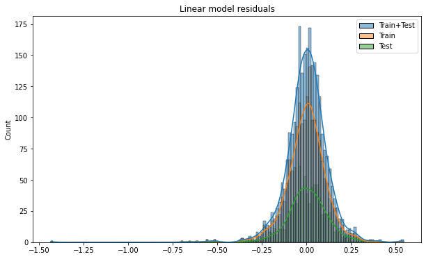
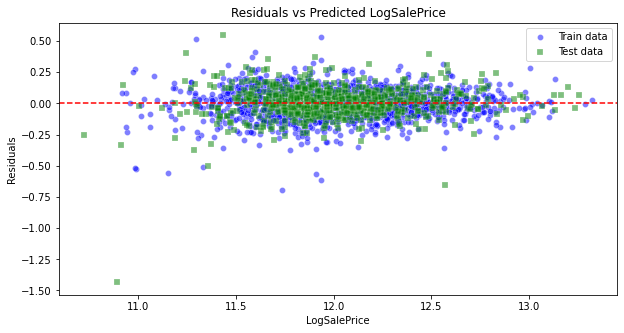
- Homoscedasticity–the residuals have constant variance
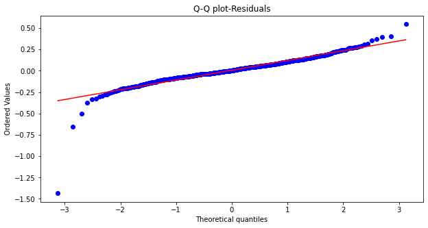
- Normality–the residuals are normally distributed
The following shows ways we checked the assumptions of multiple linear regression. We paid special attention to not inflate VIF by introducing multicollinearity when adding new features during feature selection.
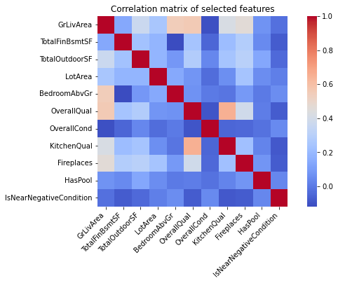
First, from the correlation matrixThe image is illustrative, we did not use these exact features in our linear model., we see that there is low multicollinearity between features.
We see that the residuals are normally distributed.
We see that the residuals are linear.
We see that the residuals are linear.
The Variance Inflation Factor (VIF) quantifies the severity of multicollinearity in regression analysis. It provides an estimate of how much the variance of a regression coefficient is increased because of collinearity. The table below shows a low generalized VIF for our predictorsWe use the
Rcarpackage'sviffunction.
| vif(model) | VIF | df | VIFdf⁄2 |
|---|---|---|---|
| GrLivArea | 4.4 | 1 | 2.10 |
| TotalFinBsmtSF | 1.57 | 1 | 1.25 |
| TotalOutdoorSF | 1.39 | 1 | 1.18 |
| LotArea | 1.48 | 1 | 1.22 |
| BedroomAbvGr | 2.33 | 1 | 1.53 |
| MSSubClass | 98.42 | 14 | 1.18 |
| MSZoning | 37.02 | 6 | 1.35 |
| OverallQual | 3.42 | 1 | 1.85 |
| OverallCond | 1.48 | 1 | 1.22 |
| Neighborhood | 2261.42 | 27 | 1.15 |
| KitchenQual | 2.2 | 1 | 1.48 |
| SaleCondition | 1.51 | 5 | 1.04 |
| YrSold | 1.21 | 4 | 1.02 |
| CentralAir | 1.51 | 1 | 1.23 |
| Fireplaces | 1.72 | 1 | 1.31 |
| HasPool | 1.06 | 1 | 1.03 |
| IsNearNegativeCondition | 1.12 | 1 | 1.06 |
| LandContour | 1.87 | 3 | 1.11 |
Table 3. Generalized vif with values mostly under 2
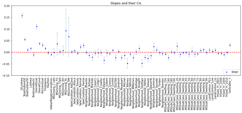
- By looking at the predictor slopes and their confidence intervals, we see that some encompass 0.
HasPoolwas thus removed as a predictor.
Realtor Recommendations
The most simple model, multiple linear regression, has benefits in that it is easily explainable. We see that by changing a feature by 1-unit, there is a positive or negative effect on SalePrice. This is useful for a realtor as they might be able to recommend a client install central air conditioning should they find a good deal on installation.
| Feature | Expected Cost | Sale Price Increase |
|---|---|---|
GrLivArea | NA | $57⁄ft2 |
BsmtLivArea | NA | $22⁄ft2 |
| Finished outdoor space | NA | $11⁄ft2 |
| Installing a fireplace | $2-5K | $4,380 |
| Installing central air | $3-15K | $23,599 |
| Near railroad | NA | -$7,675 |
Table 4. Effect of 1-unit change on mean SalePrice
Conclusion
We achieved our aim of providing value for the (fictitious) realtors in our organization through our data analysis and predictive modeling. The insights and predictions can be surfaced through a Regression Realty app so that an agent can see recommendations for renovating or setting a sale price on a particular house.
Our fictitious firm would provide us access to MLS listings, which would be incorporated into the app. Unfortunately, MLS data is not publicly available, so we could not include it in our analysis.This would cut down on the number of features a realtor would have to manually enter into our app, as the data would be auto-populated wherever possible from MLS.
Future Development
If we had more time, we would have liked to
- Use log-log transformations for our models,
- Create a mobile app for our fake realtors at Regression Realty
- Incorporate household income and MLS data into our models
- Investigate the impact of distance from Iowa State University or other locations
- This is not promising as we can see from the maps that
YearBuiltwould trump distance from a major location
- This is not promising as we can see from the maps that
- Add interaction and polynomial features
 For instance, some
 Quality features appear to be quadratic
Engineering Process
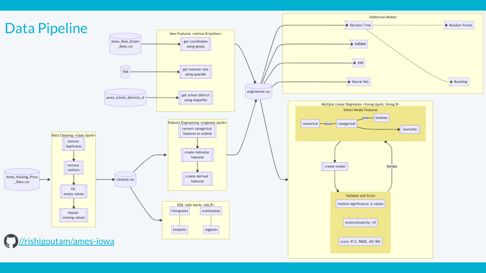
We tackled this project together with team members taking on different models. The data pipeline is shown below. Note that we would have liked to have a train-test split that was the same across all models, but did not have time to implement that. As a result, the model results are not directly comparable.
References
Ames, Iowa: Alternative to the Boston Housing Data as an End of Semester Regression Project
http://jse.amstat.org/v19n3/decock.pdf
Treasury Yields (TNX)
Ames City Neighborhoods
Ames School Districts (boundaries, shapefile)
Lillicrap, T. P. et. al., “Backpropagation and the brain”. Nat. Rev. Neurosci. 21, 335-346 (2020)